%%javascript
Jupyter.keyboard_manager.command_shortcuts.remove_shortcut('up');
Jupyter.keyboard_manager.command_shortcuts.remove_shortcut('down');
from IPython import display
Imports ..
import matplotlib.pyplot as plt
import numpy as np
from mpl_toolkits.mplot3d import Axes3D
from mpl_toolkits.mplot3d import axes3d
import pandas as pd

from rotate import rotanimate
import matplotlib.animation as animation
import subprocess
from IPython.display import Image

from matplotlib import cm
from IPython.display import Video
from sklearn.linear_model import LinearRegression
from sklearn.preprocessing import scale
plt.style.use('seaborn-whitegrid')

plt.rcParams["figure.figsize"] = [10,6]

#import numpy as np
#import matplotlib.pyplot as plt
#from mpl_toolkits.mplot3d import Axes3D
from sklearn import decomposition
from sklearn import datasets
from sklearn.preprocessing import StandardScaler

from itertools import chain
import math

import seaborn as sns; sns.set() # styling

from functools import reduce
import functools
import operator

from numpy.polynomial import polynomial as P

from scipy.interpolate import CubicSpline
from scipy.interpolate import interp1d


#### Defaults
sns.set_style("darkgrid", {"axes.facecolor": ".9"})
plt.rcParams.update({'font.size': 12})
import seaborn as sns; sns.set() # styling
Functions
def foldl(func, acc, xs):
  return functools.reduce(func, xs, acc)

# tests
#print(foldl(operator.sub, 0, [1,2,3])) # -6
#print(foldl(operator.add, 'L', ['1','2','3'])) # 'L123'

def scanl_plus(data):
    '''
    returns list of successive reduced values from the list (see haskell foldl)
    '''
    return [0] + [sum(data[:(k+1)]) for (k,v) in enumerate(data)]

def make1D (data):
      return np.array(list(map (lambda x : [x],data)))

def celsius_to_fahr(temp):
    return 9/5 * temp + 32

def gen_answers_from_alphas(inputs, new_alphas):
  return (np.matmul(inputs,new_alphas))


def polyfitx(x, y, degree):
    results = {}

    coeffs = np.polyfit(x, y, degree)

     # Polynomial Coefficients
    results['polynomial'] = coeffs.tolist()

    # r-squared
    p = np.poly1d(coeffs)
    # fit values, and mean
    yhat = p(x)                         # or [p(z) for z in x]
    ybar = np.sum(y)/len(y)          # or sum(y)/len(y)
    ssreg = np.sum((yhat-ybar)**2)   # or sum([ (yihat - ybar)**2 for yihat in yhat])
    sstot = np.sum((y - ybar)**2)    # or sum([ (yi - ybar)**2 for yi in y])
    results['determination'] = ssreg / sstot

    return results

def showECResults (title,ec_alphas, actual_alphas, principle_vals,ans, ans_scaler):
    AxH2 = principle_vals.dot (ec_alphas)
    new_nnAnsH2 = ans_scaler.inverse_transform (AxH2)
    rH2 = np.corrcoef(ans,(new_nnAnsH2.reshape(-1,)))
    rSq = (rH2[1,0])**2
    print(rSq)
    fig, ax = plt.subplots(1,2)
    ax[0].plot(ans,new_nnAnsH,'o', color='green',marker=".", markersize=1);
    ax[1].plot(ec_alphas, color='green',marker=".", markersize=10);
    ax[1].plot(actual_alphas, ':o', color='orange',marker=".", markersize=12);
    fig.suptitle(title)
    plt.show()

def left_inverse (m ):
    return (np.linalg.solve (m.T.dot(m), m.T))

# Two ways to compute this ..
# rsq = 1 - residual / sum((y - y.mean())**2)
#or
# rsq = 1 - residual / (n * y.var())
# https://stackoverflow.com/questions/3054191/converting-numpy-lstsq-residual-value-to-r2
def lstsq_rsq (output_from_lstsq, inputs, answers):
    rsq_ = 1 - output_from_lstsq[1] / sum ((answers - answers.mean())**2)
    return (rsq_[0])

def drawVector (origins,vectors):
    vectors_np = np.array(vectors)
    #origins = ([[0,0],[0,0]])
    V = vectors_np
    origins_t = zip(*origins)

    fig, ax = plt.subplots()
    fig.set_size_inches(8,8)
    origins_l = np.array(list(map(lambda t: list(t),origins_t)))

    q = ax.quiver(*origins_l, (list(V[:,0])), (list(V[:,1])), color=['r','b','g','r'], scale=1,units='xy')
    ax.set_aspect('equal')
    lim = 7
    plt.xlim(-lim,lim)
    plt.ylim(-lim,lim)

    plt.title('Vector Tutorial',fontsize=10)

    #plt.savefig('savedFig.png', bbox_inches='tight')
    #print (type(q))

    plt.show()


def splineCoeffsToAns (title,c,actual_sol, scaleF):
    plen = 5
    d = 0.3   #0.3 was this value ????
    xa = np.linspace (  0,  d,plen)
    xb = np.linspace (  d,2*d,plen)
    xc = np.linspace (2*d,3*d,plen)
    xd = np.linspace (3*d,4*d,plen)
    xe = np.linspace (4*d,5*d,plen)
    xf = np.linspace (5*d,6*d,plen)
    xg = np.linspace (6*d,7*d,plen)
    xh = np.linspace (7*d,8*d,plen)
    xi = np.linspace (8*d,9*d,plen)
    #xj = np.linspace (9*d,2,100)

    f1d = list(map (lambda xp : c[0][0]   + c[0][1]*xp  + c[0][2]*xp**2  + c[0][3]*xp**3,xa))
    f2d = list(map (lambda xp : c[1][0]   + c[1][1]*xp  + c[1][2]*xp**2  + c[1][3]*xp**3,xb))
    f3d = list(map (lambda xp : c[2][0]   + c[2][1]*xp  + c[2][2]*xp**2  + c[2][3]*xp**3,xc))
    f4d = list(map (lambda xp : c[3][0]   + c[3][1]*xp  + c[3][2]*xp**2  + c[3][3]*xp**3,xd))
    f5d = list(map (lambda xp : c[4][0]   + c[4][1]*xp  + c[4][2]*xp**2  + c[4][3]*xp**3,xe))
    f6d = list(map (lambda xp : c[5][0]   + c[5][1]*xp  + c[5][2]*xp**2  + c[5][3]*xp**3,xf))
    f7d = list(map (lambda xp : c[6][0]   + c[6][1]*xp  + c[6][2]*xp**2  + c[6][3]*xp**3,xg))
    f8d = list(map (lambda xp : c[7][0]   + c[7][1]*xp  + c[7][2]*xp**2  + c[7][3]*xp**3,xh))
    f9d = list(map (lambda xp : c[8][0]   + c[8][1]*xp  + c[8][2]*xp**2  + c[8][3]*xp**3,xi))
    #f10d = list(map (lambda xp : c[9][0]   + c[9][1]*xp  + c[9][2]*xp**2  + c[9][3]*xp**3,xj))

    ecAns = (f1d+f2d+f3d+f4d+f5d+f6d+f7d+f8d+f9d) #+f10)
    ecAnsNP = (np.array (ecAns))*-1
    print (f1d[0],f5d[0])

    subsample_sol = np.array(actual_sol[::6])
    fig9, ax9 = plt.subplots()
    ax9.set_title ("EC vs Actual -> " + title)
    ax9.plot(ecAnsNP,':o', color = "orange",markersize = 4,label="EC Sol")
    ax9.plot(subsample_sol*scaleF, ':o',markersize = 4, label = "Known Sol")
    ax9.plot ([0,plen,2*plen,3*plen,4*plen,5*plen,6*plen,7*plen,8*plen],
                [f1d[0],f2d[0],f3d[0],f4d[0],f5d[0],f6d[0],f7d[0],f8d[0],f9d[0]], 'o', color = "red", label = "EC Spline Pos")
    ax9.legend()
    #ax9.set_xlabel(r'$\Delta_i$', fontsize=15)
    #ax9.set_ylabel(r'$\Delta_{i+1}$', fontsize=15)
    #ax9.set_title('Volume and percent change')
    ax9.set_xlabel( 'Pseudo Wavelength')
    plt.savefig(title + ".png")
# Reduce Example
#reduce(lambda a,b: a+b, [1,2,3,4,5], 0)b
#display.Image("stable01.png",width=120)
Load Cell Electroincs Overview
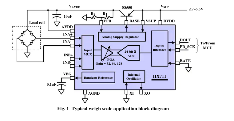
The HX711 seems to do the job, but as has been demonstated it's the details that are important. More sophisticated chips address some of these issues outlined below.
- Load cell drift
- Load cell self heating
- ADC offset error
- ADC offset drift
- ADC Gain error
- ADC Gain drift
Currently we are using the HX711 .. What else is out there, and what's the landscape ..
Competition
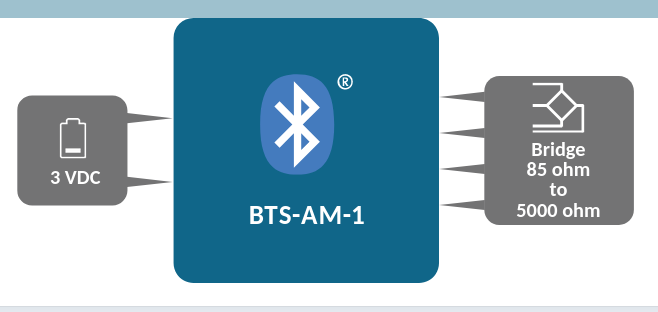 From a company called Interface,
" The BTS-AM-1 is a Bluetooth Low Energy (BLE) strain bridge transmitter module \$230.00 to \\$340.00 "
They have an intersting device .. It contains all the electronics except the load cell.
- Inputs: 3V, and 4 wire load cell
- Output: Bluetooth
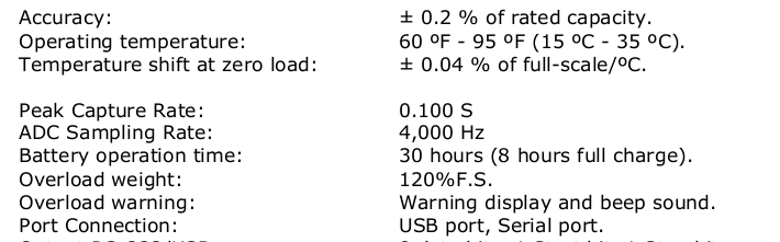
 Here are the detailed specs, i.e. Things we should be aware of.
They mention ADC drift and offset which we will see the TI RYO (roll your own) chips address.
Note the 10 month battery life on two AA cells in the spec above ..
Let's do the calcs, 2.8AH for AA's at low discharge rate, once per sec for 10 months. If we assume that the 'sleep' current is zero we get,
On_secs = 3600*24*30*10
On_hours = On_secs / 3600
Batt_capacity = 2.8 *3600  # amp-secs
On_current = Batt_capacity / On_secs
print ("Average On Current -> %d microamps" % (On_current*1e6))
#print (On_hours)
A little hard to believe. They claim a peak current of 30ma. The best battery I could find could only give about 600 service hours at that approximate discharge rate which translates into a calendar month. Also, alkalines have a self discharge rate of 3% per month.
Nextec
Main product specifications at right. No hardware sampling rate given. Only at user level of 100ms.
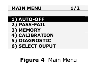
They have some additional functionality .. i.e. Production Pass/Fail.

They have another product .. Connects to scale via RS-232 / USB ?
Electronics
Avia
Overview
- +/- 20mv at 128 gain
- 10/80 SPS
- 60hz rejection
- 1.5ma / \< 1ua standby
- No differential voltage reference
- No ACload cell exitation
TI
TI has several solutions for load cell applications. They can be divided into two categories,
Roll Your Own (RYO)- Assemble the electronics from blocks, i.e. PGA (programmable gain amplifier), A/D converter, Serial Interface, etc
- ADS1235 - AC exitation and DAC, 24-bit, 7.2-kSPS
- ADS1261 - AC exitation and DAC, 24-bit, 40-kSPS
- UCC27523 - FET load cell drivers
One Chip - Similar to the HX711, but generally includes their MSP430 CPU with 'special' peripherals. There are over 400 variations.
- ADS1232/ADS1234 about \$7.
- MSP430F42 about \$4
- MSP430F449 .. no A/D
Reference Designs
Application Briefs
Perhaps the real question is does the RYO option provide a better product.
It looks like the MSP430F42xA has.
- A lower quality PGA (only 32x) than the RYO,
- No AC Exitation
- No Differential Reference Voltage.
Links:
AC Exitation (ADS1235, ADS1261, UCC27523)
MSP430F42xA App Note
ADS1232 Ref Design
ADS1232 White Paper
ADS1232 Chip
 From a company called Interface,
 From a company called Interface,
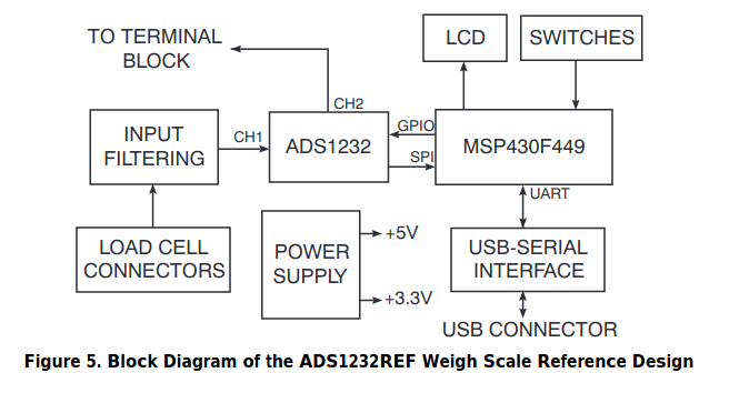
ADS1232 Reference Design Block Diagram
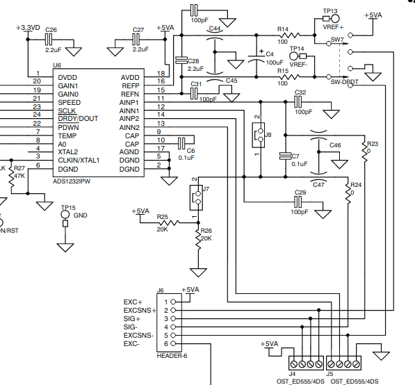
ADS1232 Reference Design input conditioning.
Quick Note on the ADS1235 vs ADS1261 ..
sample_rate_improvement = math.sqrt (40/7.2)
db_improvement = 20 * math.log10(sample_rate_improvement)
print ("Improvement with high sample rate ADS1261 (above)-> %2.0d db" % (db_improvement))
ADS1261
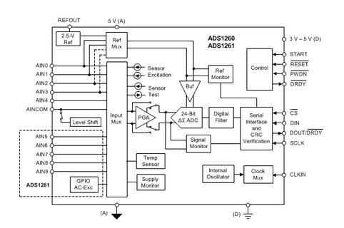 ADS1261 with AC excitation.
Analog Devices

AD7175-2 Specifications
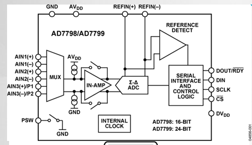
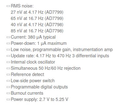
AD7799 Specifications
Note the 470 SPS and the use of a delta-sigma converter.
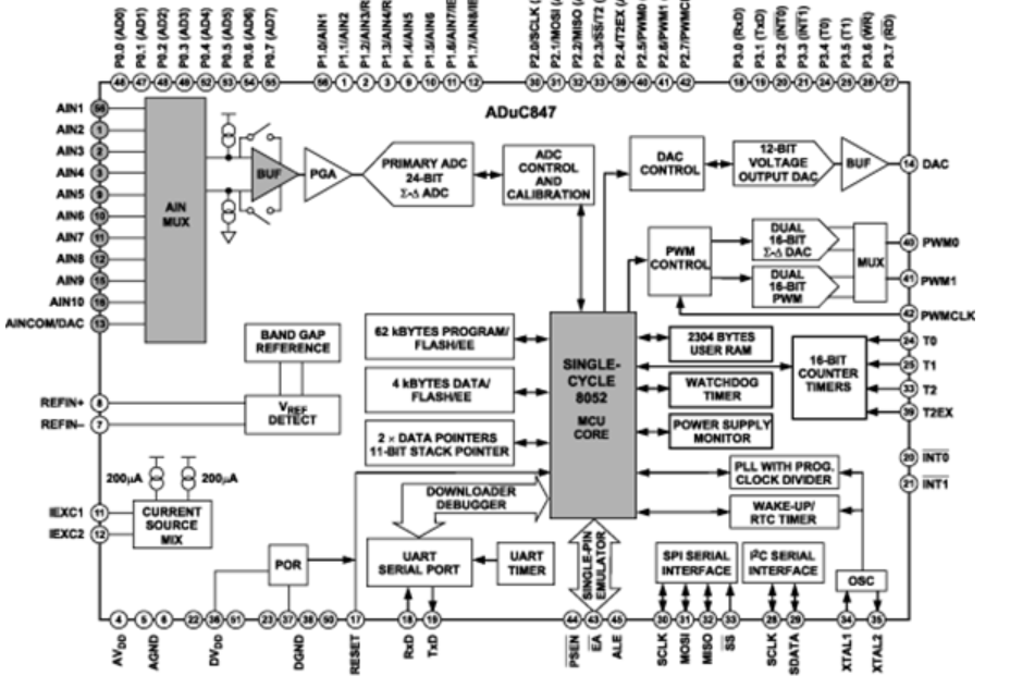
display.Image("adcuc847_bigblock.png",width=700)

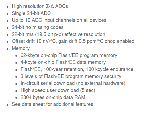
ADuC847 Specifications
Stopped ...